In this tutorial you will use ENVI Deep Learning to learn the steps necessary to train multiple models to work together to optimize classification results. By optimizing classification results, you save processing time and reduce false positives with the upfront cost of training two models. You will train two models, then use them together during classification to quickly and accurately identify small boats. This tutorial introduces a new concept to ENVI Deep Learning referred to as grid. You will train a grid model, a pixel segmentation model, and perform optimized pixel classification. The tutorial workflow is compatible with ENVI Deep Learning version 4.0 and higher.
This tutorial requires a separate installation and license for ENVI Deep Learning; contact your sales representative for more information.
See the following sections:
System Requirements
Refer to the System Requirements topic.
Files Used in This Tutorial
Sample data files are available on our ENVI Tutorials web page. Click the Deep Learning Grid link in the ENVI Tutorial Data section to download a .zip file containing the data. Extract the contents to a local directory. The training files are located in Grid_Tutorial_Data\Training\ under the TrainingRasters and ValidationRasters folders. The classification files are located in Grid_Tutorial_Data\Classification\ under the Models and Rasters folders.
|
File |
Description |
|
lr_arizona_1.dat_504060763.dat
|
Training raster - 1186-point labels
|
|
lr_arizona_2.dat_1183416481.dat
|
Training raster - 140-point labels
|
|
lr_arizona_3.dat_1776398521.dat
|
Training raster - 26-point labels
|
|
lr_arkansas_1.dat_1851476897.dat
|
Training raster - 252-point labels
|
|
lr_california_1.dat_716193635.dat
|
Training raster - 3146-point labels
|
|
lr_florida_2.dat_1259155206.dat
|
Training raster - 168-point labels
|
|
lr_florida_3.dat_1437749265.dat
|
Training raster - 8-point labels
|
|
lr_florida_5.dat_1837160688.dat
|
Training raster - 472-point labels
|
|
lr_louisiana_1.dat_944963123.dat
|
Training raster - 180-point labels
|
|
lr_maryland_1_20150815.tif_1692374196.dat
|
Training raster - 603-point labels
|
|
lr_maryland_2.dat_1024726813.dat
|
Training raster - 671-point labels
|
|
lr_missouri_1.dat_1727037987.dat
|
Training raster - 452-point labels
|
|
lr_new_hampshire_1.dat_833661639.dat
|
Training raster - 514-point labels
|
|
lr_new_hampshire_2.dat_1081387608.dat
|
Training raster - 552-point labels
|
|
lr_new_jersey_1.dat_1921660257.dat
|
Training raster - 113-point labels
|
|
lr_new_jersey_3.dat_1141542381.dat
|
Training raster - 57-point labels
|
|
lr_new_york_1.dat_1375301916.dat
|
Training raster - 156-point labels
|
|
lr_new_york_2.dat_1978166886.dat
|
Training raster - 32-point labels
|
|
lr_texas_1.dat_2115969208.dat
|
Training raster - 23-point labels
|
|
lr_washington_1.dat_1859386567.dat
|
Training raster - 2-point labels
|
|
lr_florida_1.dat_957762618.dat
|
Validation raster - 18-point labels
|
|
lr_florida_4_subset_20100503.dat_819150081.dat
|
Validation raster - 604-point labels
|
|
lr_massachusetts_2.dat_1824956166.dat
|
Validation raster - 1046-point labels
|
|
lr_new_hampshire_3.dat_554026565.dat
|
Validation raster - 409-point labels
|
|
lr_new_jersey_2.dat_664689384.dat
|
Validation raster - 110-point labels
|
|
california_1_subset_20090623.dat
|
Classification raster
|
|
florida_4_subset_20100503.dat
|
Classification raster
|
|
maryland_1_20150815.tif
|
Classification raster
|
|
massachusetts_1_20100821.tif
|
Classification raster
|
|
TrainedGridModel.envi.onnx
|
Single class 100-epoch model
|
|
TrainedPixelModel.envi.onnx
|
Single class 25-epoch model
|
Background
The Grid tutorial dataset was constructed using data from the National Agriculture Imagery Program (NAIP). NAIP is public domain data and freely accessible. For more information regarding the data, see https://www.fsa.usda.gov/Assets/USDA-FSA-Public/usdafiles/APFO/support-documents/pdfs/naip_infosheet_2017.pdf.
The training dataset provided with this tutorial contains rasters collected over 14 states, providing different regions with boat features. The dataset was pre-labeled and made ready for training. Labels were hand-selected in 20 rasters totaling 8753 labeled points for training, and 5 validation rasters totaling 2187 points. The total number of labeled points is 10,940, data was split between training and validation with roughly 80% for training, and 20% for validation. Point labels represent a single pixel centered on the target feature, for this dataset the features are boats.
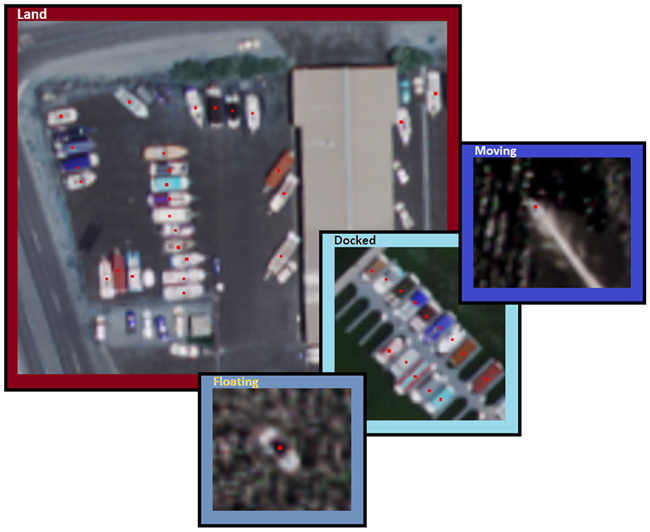
A single boat class was used for all labels in the dataset, multiple views of the feature were labeled. In the example image below, from training raster lr_arizona_1.dat_504060763.dat, you can see points over boats on land, floating, docked, and moving in open water. All boats were labeled using the ENVI Deep Learning Labeling Tool.
Additional data includes four rasters for classification, to see how well the models generalizes on data that was not used during training.
During the training process, all labeled data is viewed by the algorithm once per epoch. The definition of an epoch is one complete cycle through the training dataset. At the end of each epoch, validation data is compared against what the model has learned from the training data.
Train a Deep Learning Grid Model
Trained Grid models provide tipping and cueing to scan a raster and detect locations with potential features of interest quickly. A grid model can be used for classification on its own, or the grid classification can be used as input to optimized pixel segmentation and optimized object detection classifications to speed up processing. Grid training supports both pixel segmentation label rasters, and object detection label rasters. This tutorial will guide you through the process using pixel segmentation label rasters.
To easily reference generated content, create a folder where you have access using the name Grid_Tutorial_Output. This location will be referenced throughout the tutorial.
- Start ENVI.
- In the ENVI Toolbox, select Deep Learning > Grid > Train Deep Learning Grid Model The Train Deep Learning Grid Model dialog appears with the Main tab selected.
- Click the Add Files button
 next to the Training Rasters field and select all training raster files provided with the tutorial data under Grid_Tutorial_Data\Training\TrainingRasters.
- Click the Add Files button next to the Validation Rasters field and select all validation raster files provided with the tutorial data under Grid_Tutorial_Data\Training\ValidationRasters.
- In the Output Model field, click the Browse button
 , navigate to the Grid_Tutorial_Output folder, and name the output model BestGridModel.envi.onnx.
- In the Output Last Model field, click the Browse button, navigate to the Grid_Tutorial_Output folder you created, and name the output model LastGridModel.envi.onnx.
-
Select the Model tab, then set the parameters as follows:
-
Name: NAIP Boats Grid
-
Description: Leave blank
-
Architecture: ResNet50
-
Grid Size: 448
The grid size of the model matters when paired with another model for optimized classification. Grid size must be a multiple of 32 with a minimum size of 224 squared. The patch size used in the next section, Train a Deep Learning Pixel Model, is set to the default 464.
When running optimized classification, the grid will target areas of 448x448 containing features. Pixel classification will target features within the grid cell and extend outward by 16 pixels outside the grid boundary. This feature allows the pixel classifier to identify features on the outer boundary of the grid cells.
The following illustration shows a grid cell size of 224 (green) and a patch size of 464 (black). Pixel patches of patch size are center over grid cells of grid size. When running an optimized classifier, the pixel model will extend 120 pixels outside the grid targeted area. Doing this allows for potential false positives beyond the grid location, but could also provide classification context beyond the grid for features on the edge of the grid cell. Limiting the extent of the patch size to 16 or 32 pixels outside the grid can improve classification results by reducing false positives.

-
Select the Training tab, then set the parameters as follows:
- Augment Scale: Yes
- Augment Rotation: Yes
- Number of Epochs: 100
- Patches per Batch: 5 (can be increased for GPUs with memory greater than 8GB)
- Feature Patch Percentage: 1.0
-
Background Patch Ratio: 0.7
Background patch ratio provides control over the number of patches without class features that are viewed by the algorithm during training. Due to boats appearing similar in shape and color with other features in the data, a value of 0.7 is used. Adding background data helps grid differentiate better between boats and background. For example, a value of 0.7 uses 70 background patches for every 100 patches with features.
Examples:
|
Ratio
|
Feature Patches
|
Background Patches
|
|
2.0
|
100
|
200
|
|
1.0
|
100
|
100
|
|
0.5
|
100
|
50
|
|
0.0
|
100
|
0
|
-
Select the Advanced tab, then enter a Solid Distance of [6].
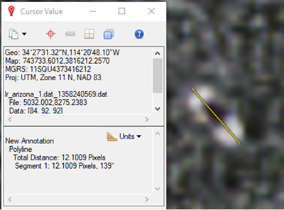
Solid distance is a patented technology adopted from the ENVI Deep Learning Pixel Segmentation training workflow. A value of 6 is based on half the average boat size in the training data. Using ENVI’s Mensuration tool you can easily determine a features size in pixels along its largest axis.
-
The Mensuration tool  is located on the right side of the ENVI toolbar. Click the icon to open the Cursor Value dialog.
-
From the Cursor Value dialog's Units drop-down list, select Pixel.
-
In the raster, click one end of a feature, then click the end of that feature that is farthest away. The Total Distance of the line displays in the Cursor Dialog. Below is an example of a boat used in this tutorial. Measuring front to back, the boat is roughly 12 pixels long. Based on the feature length, divide by two to determine the Solid Distance value, which in this case would be 6. A value of 6 is close to the average boat size and should represent the smaller dimension of your features. This means that if the Solid Distance value was set to 12 or 13, the model will not do well, particularly where boats are grouped next to each other (such as in docks).
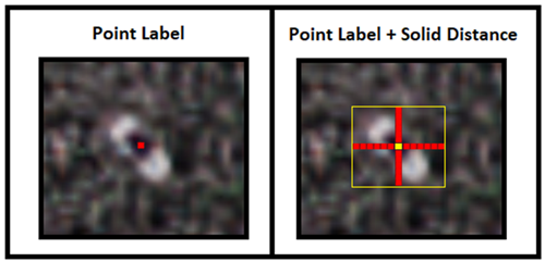
Solid distance compensates for point labels by extending a point in four directions by the number of pixels specified for solid distance. The example image below shows a standard point label comprised of a single pixel roughly centered on the feature (left) and the original point label in yellow (right), with six red pixels extending up, down, left, and right of the point. The yellow box represents the actual data viewed during training, which is a label patch with dimensions 13px * 13px * nBands.
- Set Pad Small Features to No (it is only used for object detection)
- Click OK.
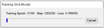
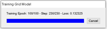
As training begins, a Training Model dialog reports the current epoch, step, and training loss, for example:
Also, a TensorBoard page displays in a web browser. TensorBoard is described in View Training and Accuracy Metrics.
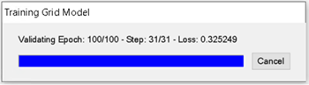
At the end of every epoch, the training progress dialog will update, providing information regarding validation. For example:
- The final step of epoch 24 training reports a loss of 0.260588, this refers to the training loss in the metrics.
- The final step of epoch 24 validation reports a loss of 0.277377, this refers to the validation loss in the metrics.
Your results will likely be different; not all training sessions report the same values for metrics due to the randomness of deep learning.
Training a model takes a significant amount of time due to the computations involved. Processing can take several hours to complete, depending on your system hardware and GPU. If you prefer not to wait that long, you can cancel the training step now and use the trained grid model (TrainedGridModel.envi.onnx) that was created for this tutorial, later in the grid classification and optimized pixel classification steps. This file is included with the tutorial data under Grid_Tutorial_Data\Classification\Models. The tutorial data provides one grid and one pixel model that were trained using the default Number of Epochs setting. The default number of epochs were used to train the model for this tutorial due to the amount of time it takes, however, the models were still converging. You could optionally train both models possibly doubling the Number of Epochs and receive better results.
Finalizing training:
Finalizing validation:
At this point, you can go through the steps to Perform Grid Classification to test your grid model. Next, you will train a Deep Learning pixel model, which is required to Perform Optimized Pixel Classification.
Train a Deep Learning Pixel Model
Pixel model training involves repeatedly exposing label rasters to a model. Over time, the model will learn to translate the spectral and spatial information in the label rasters into a classification image that maps the features it was shown during training.
- In the ENVI Toolbox, select Deep Learning > Pixel Segmentation > Train Deep Learning Pixel Model The Train Deep Learning Pixel Model dialog appears with the Main tab selected.
- Click the Add Files button next to the Training Rasters field and select all training raster files provided with the tutorial data under Grid_Tutorial_Data\Training\TrainingRasters.
- Click the Add Files button next to the Validation Rasters field and select all validation raster files provided with the tutorial data under Grid_Tutorial_Data\Training\ValidationRasters.
-
In the Output Model field, click the Browse button , navigate to the Grid_Tutorial_Output folder you created, and name the output model BestPixelModel.envi.onnx.
-
In the Output Last Model field, click the Browse button, navigate to the Grid_Tutorial_Output folder you created, and name the output model LastPixelModel.envi.onnx.
-
Select the Model tab, then set the parameters as follows:
-
Select the Training tab, then set the parameters as follows:
-
Select the Advanced tab, then set the parameters as follows:
-
Class Names: Leave blank
-
Solid Distance: [6]
-
Blur Distance: [[4, 8]]
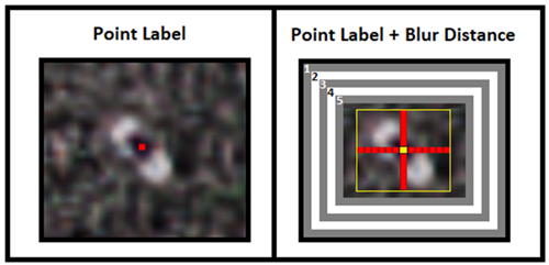
Blur distance is a patented technique for focusing the training algorithm on a feature to be learned. This is done by blurring the background around the feature once per epoch, decreasing the visible range of background around the feature. The extents of solid distance plus blur distance minimum is the end of the blurred distance, which occurs in the final epoch of training. The end of blur distance refers to the minimum value specified, in this case is 4 pixels. For this example, we blur an area around the label patch starting 8 pixels outward in all directions from the extents of the solid distance boundary. As training progresses each epoch, the blurred area around the feature is increased inwards. This continues every epoch until the final epoch reaches the blur distance minimum outside the boundary of the solid distance.
In the illustration below (left) is a labeled point over a boat included with the tutorial data. The image below (right) depicts the solid distance extent identified by the faint yellow border around the red cross. At the center of the red cross is the original point colored yellow. Solid distance extends outward by 6 pixels in all directions identified by the red cross.
The gray and white boxes represent the blur distance at each epoch. For simplicity let’s assume there are only five epochs for training. Numbers 1 through 5 in the image below represent the epoch and where blurring occurs. To visualize what happens, imagine training is in the first epoch, blur boxes 2 through 5 would not be present and appear as the regular pixels in the image. As epochs increase we focus in on the feature blurring more background as we approach the solid distance extent. Blur distance stops 4 pixels before reaching the extent of solid distance.
-
Class Weight: Min: 0.0, Max: 3.0
-
Loss Weight: 0.5
- Click OK.
As training begins, a Training Model dialog reports the current epoch, step, and training loss, for example:
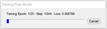
Also, a TensorBoard page displays in a new web browser. This is described next, in View Training and Accuracy Metrics.
Training a model takes a significant amount of time due to the computations involved. Processing can take several hours to complete, depending on your system hardware and GPU. If you prefer not to wait that long, you can cancel the training step now and use the trained pixel model (Grid_Tutorial_Data\Classification\Models\TrainedPixelModel.envi.onnx) that was created for this tutorial when you get to the optimized pixel classification section. The tutorial data provides one grid and one pixel model that were trained using the default Number of Epochs setting. The default number of epochs were used to train the model for this tutorial because of the amount of time it takes; however, the models were still converging. You could optionally train both models, possibly doubling the Number of Epochs, and receive better results.
View Training and Accuracy Metrics
TensorBoard is a visualization toolkit included with Deep Learning. It reports real-time metrics such as Loss, Accuracy, Precision, and Recall during training. Refer to the TensorBoard online documentation for details on how to use it.
Grid Training Metrics
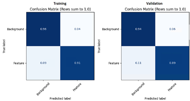
As mentioned above, both models were still converging when training completed. Looking at the grid Training and Validation Confusion Matrices in TensorBoard, you can see there is still room for improvement. Results may vary.
Background and Feature labels in TensorBoard are specific to training grid models with ENVI Deep Learning. Grid produces binary classifiers where class 0 represents background, and class 1 represents all labeled features.
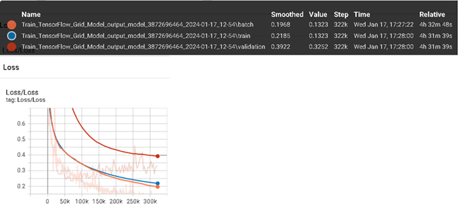
Viewing the Loss in TensorBoard, you can see it is still on a downward trend toward 0.
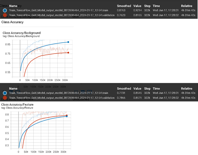
Similarly, viewing the class accuracies in TensorBoard shows they are still ascending toward 1. In the image below, Class Accuracy/Background (top) refers to everything that was not a feature. Class Accuracy/Feature (bottom), refers to the accuracy of all features learned, regardless of the number of classes.
Pixel Segmentation Training Metrics
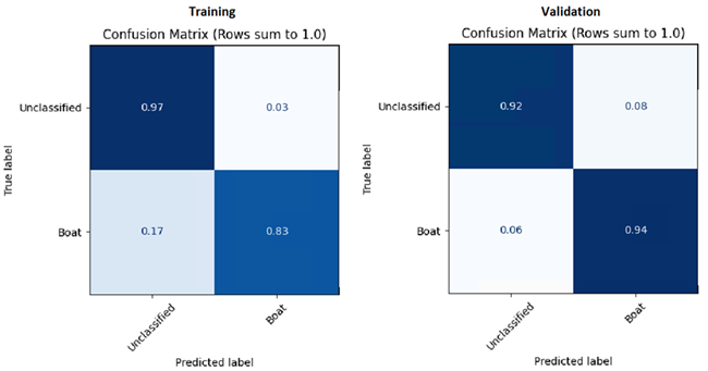
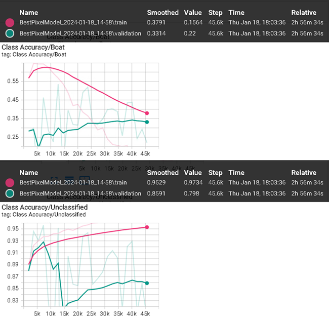
With only 25 epochs, the pixel segmentation matrices look decent, showing the model is converging. Parameter tuning and a longer training session will improve the overall model for classification. Notice the Unclassified and Boat labels in the image below. Unclassified represents class 0 or unlabeled background. Boat represents the labeled data class for this dataset.
Viewing the loss value for pixel segmentation you will see validation is a bit jumpy. Training loss is still descending, meaning this model was still learning and has room for improvement.
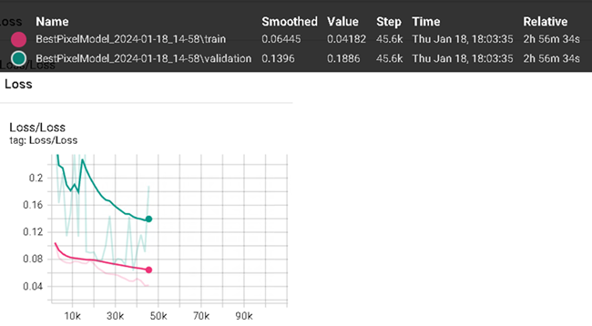
Viewing the accuracies for pixel segmentation in an example run, the results do not look as promising. The model appears to be having a difficult time accurately identifying boats vs background. Something to note is that not all training sessions are equal; different sessions can result in significantly different outcomes.
In the image below, class accuracy for boat is declining for training and slowly increasing for validation. While unclassified is ascending, background data for this example is easier to learn than the single boat class.
A breakdown of boat pixels used during training can help understand why this is a hard problem to converge on. The table below does not account for validation pixels, only pixels used during training.
|
Variable |
Value |
Calculation |
|
Training Point Labels
|
8754 Pixels |
N/A |
|
Number of Bands |
4 Bands |
N/A |
|
Solid Distance |
6 Pixels |
6 * 2 + point (1)
|
|
Expanded Point Labels
|
676 Pixels |
13 * 13 * 4 |
|
Training Pixels |
5,917,704 Pixels
|
676 * 8754 |
The number of pixels the model receives for training is less than a raster with the dimensions 1220 * 1220 * 4 (which is 5,953,600 pixels). While this might sound like a lot of information, for deep learning it is not. Adding additional labeled data, tinkering with Solid Distance and Blur Distance settings, training longer, or introducing a small amount of background data might help improve this model.
With small features and minimal data, as long as loss is going down and the confusion matrices report real features, they usually do a good job.
Now that you have trained a grid model and a pixel model, the next step is to perform grid classification.
Perform Grid Classification
You can use grids two ways to process an image. The first method is to directly classify an image with a single grid model, which generates a grid showing likely locations where your features of interest exist in the scene. The second method is to use a grid model combined with either an object detection or segmentation model to perform optimized classification. The second method is demonstrated later in this tutorial.
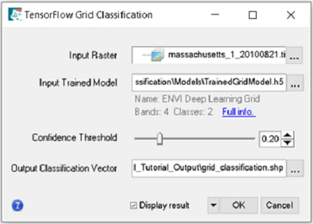
- In the ENVI Toolbox, select Grid > Deep Learning Grid Classification. The Deep Learning Grid Classification dialog appears.
- In the Input Raster field, click the Browse button , navigate to the Grid_Tutorial_Data\Classification\Rasters folder and select the raster you want to classify. The results detailed in this section will be based on the tutorial data raster Grid_Tutorial_Data\Classification\Rasters\massachusetts_1_20100821.tif.
-
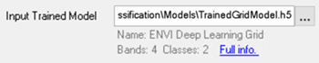
In the Input Model field, click the Browse button . The Select Deep Learning ONNX Model dialog appears. Click Open, navigate to the Grid_Tutorial_Output folder, and select BestGridModel.envi.onnx, the grid model you trained earlier in this tutorial. The results detailed in this section will be based on the grid model provided with the tutorial data Grid_Tutorial_Data\Classification\Models\TrainedGridModel.envi.onnx.
You can optionally, click the Full info link below the Input Model field to see training metadata.
-
Set the remaining parameters as follows:
-
Confidence Threshold: 0.2. Grid cells with a confidence score less than this value will be discarded. Decreasing this value generally results in more classification grid cells throughout the scene. Increasing it results in fewer classification grid cells.
Starting with a low confidence threshold is recommended to determine how well the model will do during classification. You can later rerun classification with a suitable confidence value that best identifies features.
-
Processing Runtime: CUDA. This parameter supports running on an NVIDIA GPU by default which is recommended. CPU, the other option, provides support for non-GPU enabled systems. Leave the default as CUDA unless you need to change it.
-
CUDA Device ID: Leave this parameter blank. If a valid GPU is detected then it will default to GPU ID 0. If your system contains multiple NVIDIA GPUs, you can set the appropriate ID for the GPU to host processing (leave the field blank or specify 0 for the first GPU).
-
Output Classification Vector: Optionally, click the Browse button , navigate to the Grid_Tutorial_Output folder you created and enter grid_classification.shp, then click Save. A temporary vector file will be created if not specified.
-
Enable the Display result option.
-
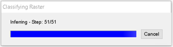
Click OK. A Classifying Raster progress dialog shows the status of processing.
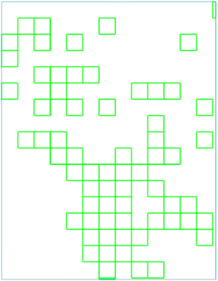
When classification completes, the grid classification output vector displays in ENVI.
-
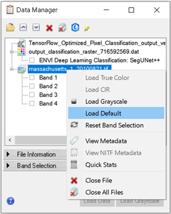
Load the raster into the view and overlay the grid classification vector on the raster.
-
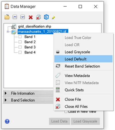
Click the Data Manager button  , in the top left of the ENVI Toolbar. Right click on the raster and select Load Default.
To help understand the results from our grid model, we can use ENVI's Filter Vector tool to interactively see how confidently grid identified boats in portions of our image. If you are making a grid model for the first time, it can be useful to set the classification confidence threshold to 0.0 and interactively use the Filter Vector tool to find a good threshold for your model and features.
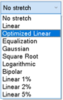
With the raster loaded in the view, select the stretch drop list, and select Optimized Linear.
In the Layer Manager, drag the raster below the grid_classification.shp file.
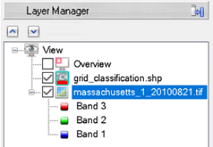
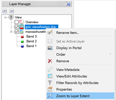
-
In the Layer Manager, right click grid_classification.shp and select Zoom to Layer Extent.
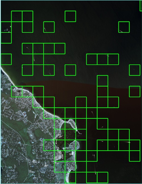
At first glance you will notice the grid cells are mostly over the water. This is good since most the boats in this scene are in the water. From this view it is hard to see any boats excluding the wake behind the boats in open waters.
To perform the cleanest classification possible, we can eliminate grid cells with lower confidence values. Also, we can learn how confident the model is for the given raster. You can do this by filtering features by confidence in ENVI.
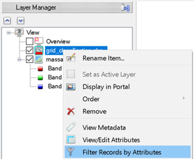
-
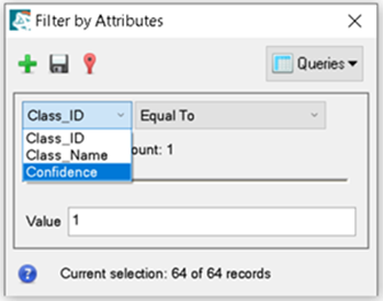
In the Layer Manager, right click grid_classification.shp and select Filter Records by Attributes. The Filter by Attributes dialog appears.
-
In the Filter by Attributes dialog, click Class_ID and select Confidence.
-
Filter by Attributes displays that there are 44 unique attribute values for confidence, and 64 records total. This means that some grid cells share the same confidence values. To easily identify cells pertaining to the selected confidence value, we will change the filter line color from black to red.
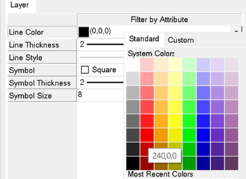
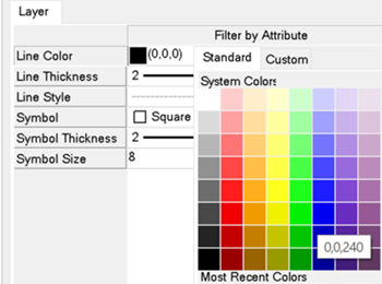
In the Layer tab below the ENVI Toolbox, select Line Color and choose a red color.
The filtered records change from black to red in the ENVI view.
-
Using the attribute slider bar, move it back and forth to discover the model’s confidence values for each feature in the raster. For example, slide the bar to 0.999 (the far right side); the boxes outlined in red are the most accurately classified features for this raster.
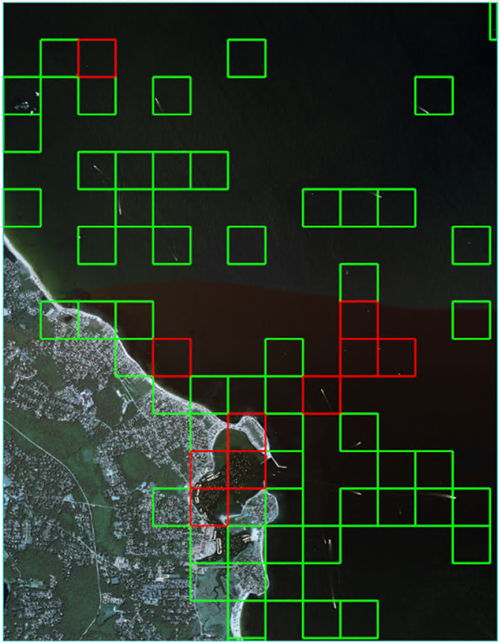
Zoom in for a closer look; there are many boats in this raster.
Perform Optimized Pixel Classification
This section steps you through how to process an image using a grid model combined with object detection or segmentation model to perform optimized classification (patent pending).
You will leverage both a trained grid model and a trained pixel segmentation model to identify small boats. Optimized pixel segmentation is the process of tipping a more advanced model such as pixel segmentation, using a grid model. Grid only knows whether a learned feature exists in portions of the grid. Pixel segmentation only knows pixel based segmentation for the features learned. Together they can quickly avoid unnecessary processing and focus on regions containing the target feature.
-
In the ENVI Toolbox, select Grid > Deep Learning Optimized Pixel Classification. The Tensor Flow Optimized Pixel Classification dialog appears.
-
In the Input Raster field, click the Browse button , navigate to the Grid_Tutorial_Data\Classification\Rasters folder and select the raster you want to classify. The results detailed in this section will be based on the tutorial data raster Grid_Tutorial_Data\Classification\Rasters\massachusetts_1_20100821.tif.
-
In the Input Trained Pixel Model field, click the Browse button . navigate to Grid_Tutorial_Output, and select the BestPixelModel.envi.onnx for the pixel model you trained earlier in this tutorial. Results for this section will be based on the pixel model provided with the tutorial data, located in Grid_Tutorial_Data\Classification\Models\TrainedPixelModel.envi.onnx.
-
In the Input Trained Grid Model field, click the Browse button . navigate to Grid_Tutorial_Output, and select the BestGridModel.envi.onnx for the grid model you trained earlier in this tutorial. Results for this section will be based on the grid model provided with the tutorial data, located in Grid_Tutorial_Data\Classification\Models\TrainedGridModel.envi.onnx.
-
Set the remaining parameters as follows:
-
Confidence Threshold: 0.6. Grid cells with a confidence score less than this value will be discarded. Decreasing this value generally results in more classification grid cells throughout the scene. Increasing it results in fewer classification grid cells.
-
Output Class Activation Raster: Enable the Display result check box to use a temporary file.
-
Output Classification Vector: Enable the Display result check box to use a temporary file.
-
Enable the Display result option.
-
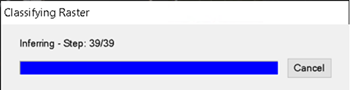
Click OK. A Classifying Raster progress dialog shows the status of processing. Optimized classification dialogs split the classification progress between grid and pixel/object classifiers.
Grid Classification progress:
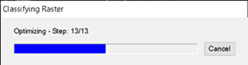
Pixel Segmentation progress:
When processing is complete, the classification result is displayed in the Image window; for example:
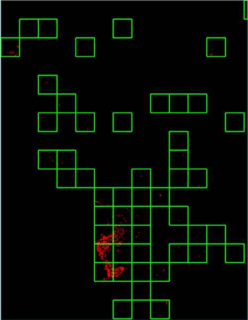
The next steps will guide you through the process of visualizing the final output of boat features with the optimized classification result.
-
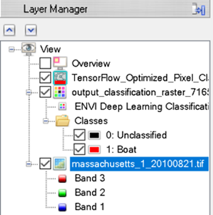
Load the raster into the view, and overlay the grid classification vector and the classification raster over the raster.
-
Click the Data Manager button , in the top left of the ENVI Toolbar. Right click on the raster and select Load Default.
With the raster loaded in the view, select the stretch drop list, and select Optimized Linear.
In the Layer Manager, drag the raster below the classification raster and vector files.
-
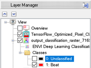
In the Layer Manager, disable the 0: Unclassified class in the classification raster by clicking to deselect the check box.
-
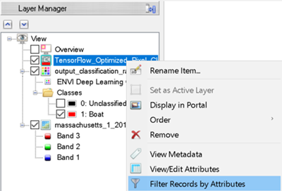
Right-click the grid vector in the Layer Manager, then click Filter Records by Attributes.
-
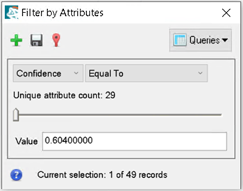
In the Filter by Attributes dialog, click Class_ID and select Confidence.
By specifying a confidence threshold of 0.6 during classification, there are fewer records than what was reported in the grid classification you performed earlier in this tutorial. The Filter by Attributes dialog reports 29 unique confidence values, and 49 grid cell detections. With a confidence threshold of 0.2, there would be 44 unique attributes and 64 total records. By increasing the confidence threshold, we eliminated less-confident detections to avoid additional false positives.
-
To easily visualize the filtered attributes by confidence value, change the line color for filtered records. Ensure Filter is selected in the Layer Manager. In the Layer tab below the ENVI Toolbox, click Line Color and change this to a blue color.
-
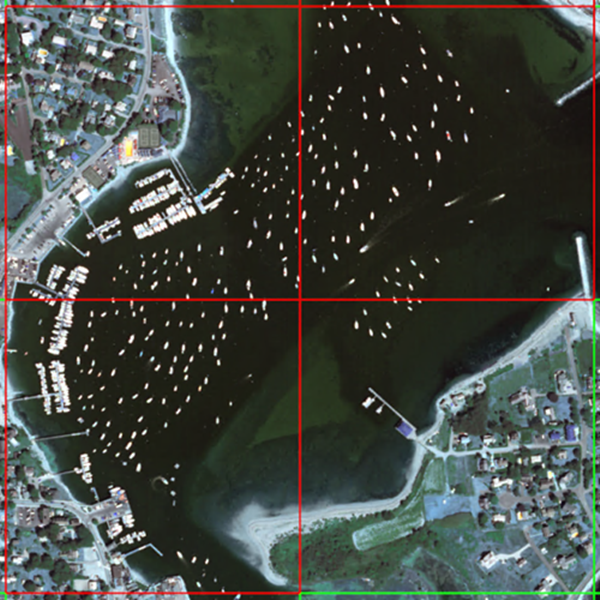
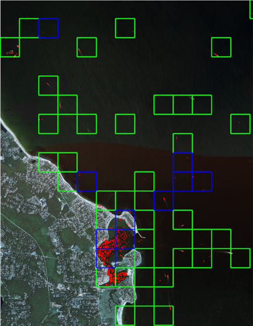
In the Filter by Attributes dialog, drag the slider to 0.999. This will show detections with the highest confidence. For example:
-
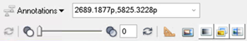
Zoom in for a closer look. In the ENVI Go To field in the Toolbar, enter the coordinates 2689.1877p, 5825.3228p and press the Enter key.
-
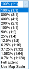
With the classification raster selected in the Layer Manager, select 100% (1:1) using ENVI’s zoom drop list.
-
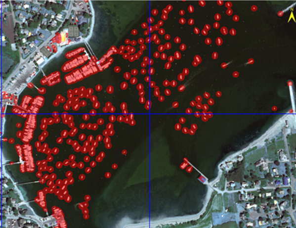
With the classification raster still selected in the Layer Manager, type 50 in ENVI’s Transparency tool.
You should now be able to see the individual boat detections below the red classification image. For example:
A final comparison between Optimized Pixel Classification and standard Pixel Classification: standard pixel classification takes longer because each portion of the image being classified is processed. For example, standard classification takes 124 steps using the same raster used above. Optimized Pixel Classification took a total of 52 steps using two models, grid 13 steps, and pixel segmentation 39 steps. More than half the processing was eliminated by leverage a grid model.
This works because grid quickly views the raster only checking to see if features exist or not in grid regions. After grid determines regions with targeted features, pixel segmentation only performs classification in those areas defined by grid.
Your result may be slightly different than what is shown here. Training a deep learning model involves several stochastic processes that contain a certain degree of randomness. This means you will never get the same result from multiple training runs.
This completes the Optimized Pixel Classification Using a Grid Model tutorial. When you are finished, exit ENVI.