The SPHERE_HARM_FORWARD function uses the Gauss-Legendre algorithm to compute the forward spherical harmonic transform of a two-dimensional input array on a spherical coordinate grid. The input latitudes should be on a Gauss-Legendre grid.
The spherical harmonic transform is a useful tool for analyzing wave patterns on a global dataset, and is extensively used in meteorology and oceanography, and in the study of geomagnetic and solar magnetic fields.
The forward and inverse transforms are also useful for applying a spectral filter. In this case, the forward transform is performed, then a filtering function is applied to the spectral coefficients, and then the inverse transform is performed.
For details on the algorithm see below.
SPHERE_HARM_FORWARD is based on the original spherical_transform routine written by Mark Miesch and modified by Marc DeRosa and Gilbert P. Compo, and is used with permission.
Example
In this example, we do a forward + inverse transform on a two-dimensional array of air temperatures from 1 Dec 1884.
restore, filepath('reanl20v3_1dec1884_512x256dbl.sav', subdir=['examples', 'data'])
ntheta = A.dim[1]
lmax = ntheta - 1
costheta = gauss_quad_legendre(-1, 1, ntheta)
B = sphere_harm_forward(A, costheta, lmax=lmax)
A1 = sphere_harm_inverse(B, costheta, lmax=lmax)
print, 'maximum error: ', max(abs(A1 - A))
IDL prints:
maximum error: 2.4930245e-09
For a more detailed example as well as data credits and reference, see below.
Syntax
Result = SPHERE_HARM_FORWARD( Array, Costheta, LMAX=value, PERIOD=value, /TPOOL_NOTHREAD)
Return Value
The result is a double-precision complex array of dimension [LMAX+1, LMAX+1], where the first dimension represents the degree l values and the second dimension represents the order m values. Because of the symmetry of the associated Legendre polynomials, the result will only have nonzero values along the diagonal and to the lower right of the diagonal. If the result is denoted by Blm, where l is the degree and m is the order, then Blm ≠ 0 for l = m...LMAX.
Arguments
Array
An input array of real values, A(φ, θ) of dimensions [nphi, ntheta], where nphi is the number of longitude points and ntheta is the number of latitude points.
Costheta
An input vector of length ntheta, containing the cosine of the theta colatitude points on a Gauss-Legendre grid. These values may be computed using the GAUSS_QUAD_LEGENDRE function, with integration limits –1 to 1.
Keywords
LMAX
Set this keyword to the maximum degree l in the expansion. The Legendre degrees will then range from 0 to LMAX, giving LMAX+1 values. The default is (2*ntheta – 1)/3.
PERIOD
Set this keyword to an integers ≥ 1 giving the periodicity of the waves in the longitudinal direction. Only Fourier coefficients that are integer multiples of the period will be computed. For example, if your data is known to be periodic in longitude, with a wavelength of 120°, then you only need to compute the spherical harmonics over a 0° to 120° swath of longitude on the sphere. In this case you would set PERIOD=3, and you would get an expansion with only mode values of m = 0, ±3, ±6, ±9, etc.
If this keyword is > 1 then the result will have dimensions [LMAX+1, (LMAX+PERIOD) / PERIOD]. The default is PERIOD=1, which will return every m value.
Note: If you set PERIOD in your initial call to SPHERE_HARM_FORWARD, you should set the same PERIOD value when calling SPHERE_HARM_INVERSE.
TPOOL_NOTHREAD
Set this keyword to explicitly prevent IDL from using the thread pool for the computation. If this keyword is set, IDL will use the non-threaded implementation of the routine even if the current settings of the !CPU system variable would allow use of the threaded implementation.
Background
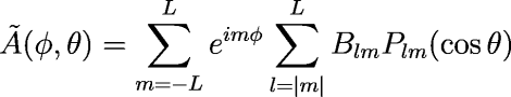
Given an input array A(φ, θ), where φ is the longitude and θ is the colatitude (90°–latitude), the value at each point can be approximated by a weighted sum of spherical harmonics:
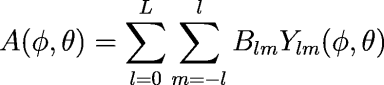
The Ylm are the spherical harmonics:
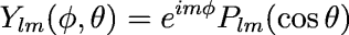
where Plm are the associated Legendre polynomials normalized for spherical harmonics. Note that the Ylm can be viewed as a set of Fourier components exp(imφ) in longitude and associated Legendre polynomials in colatitude θ.
Forward Transform
SPHERE_HARM_FORWARD computes the coefficients Blm by first computing the fast Fourier transform in the longitude direction, and then computing the Legendre transform in the latitude direction. The Legendre transform is computed using Gauss-Legendre quadrature as:
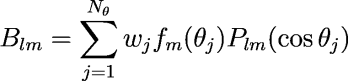
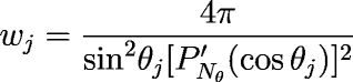
where fm are the Fourier coefficients at each latitude and wj are the appropriate weights for Gauss-Legendre quadrature. The weights wj are computed using the GAUSS_QUAD_LEGENDRE function, normalized to 4ϖ for spherical coordinates:
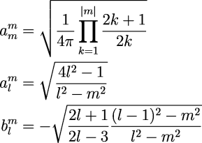
The associated Legendre polynomials Plm are computed recursively by:
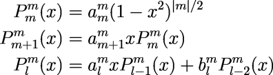
where the coefficients are:
Inverse Transform
Given a set of coefficients Blm and starting with the first equation for A(φ, θ) above, that can be rewritten as:
The inverse transform is thus an inner sum of the associated Legendre polynomials over the degree l, followed by a fast Fourier transform of the Fourier coefficients over the order m.
Note that depending upon the maximum L value (the keyword LMAX), the inverse transform result Ã(φ, θ) may not be exactly equal to the original array A(φ, θ) to the forward transform.
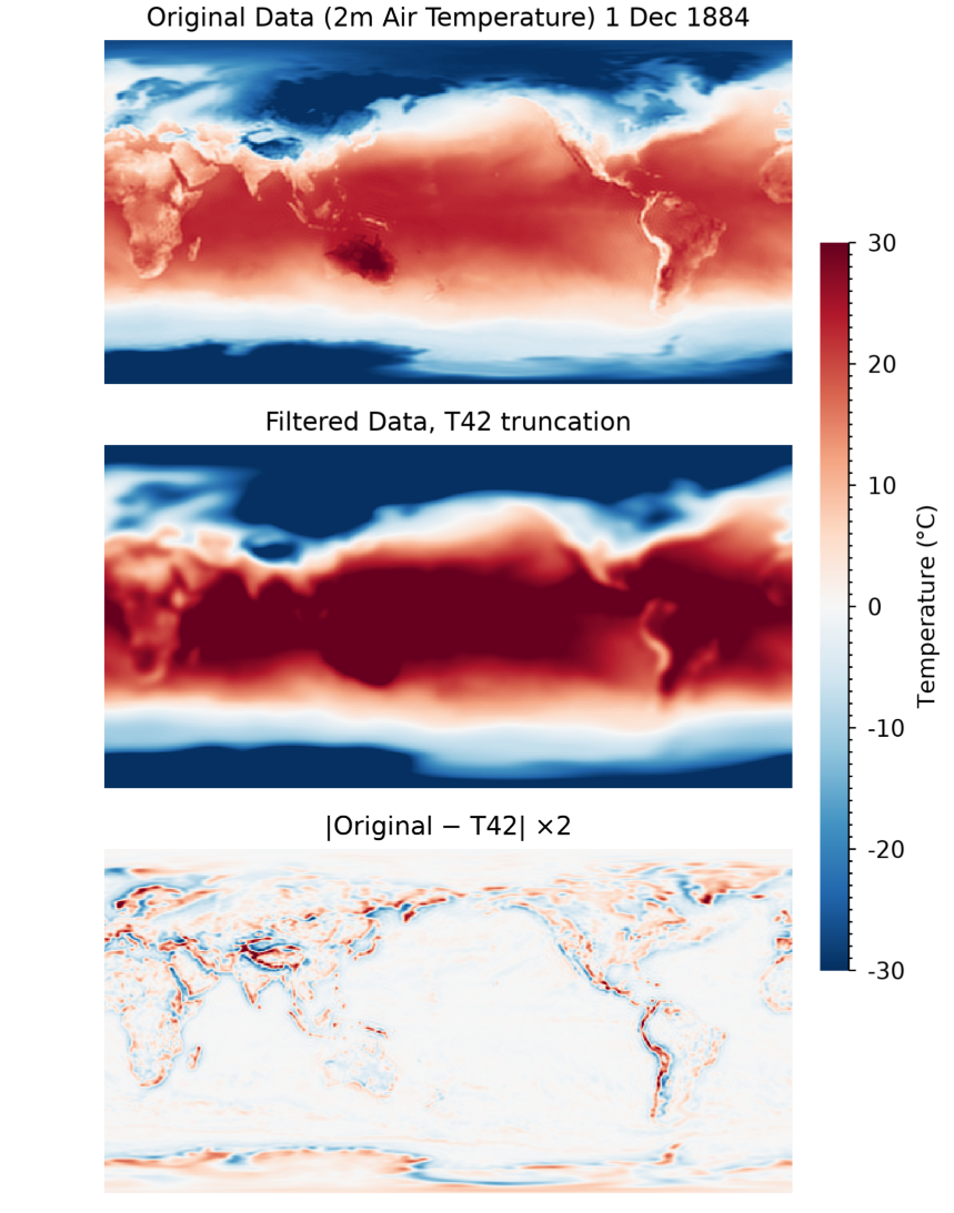
Example
In this example, we load a two-dimensional array of air temperatures from 1 Dec 1884. We then use the spherical harmonic transform to filter the data to preserve the lower frequency waves in the atmosphere. Finally, we plot the difference between the low-frequency data and the original data, which is a map of the high-frequency components.
Tip: To illustrate how to call these functions, we construct the filter kernel and perform the filter ourselves. However, you can also use the SPHERE_HARM_FILTER function to perform all of the below steps in a single function call.
 restore, filepath('reanl20v3_1dec1884_512x256dbl.sav', subdir=['examples', 'data'])
ntheta = A.dim[1]
lmax = ntheta - 1
costheta = gauss_quad_legendre(-1, 1, ntheta)
B = sphere_harm_forward(A, costheta, lmax=lmax)
filter42 = sphere_harm_kernel(lmax, 42)
Bfilter42 = B * rebin(filter42, lmax + 1, lmax + 1)
Afilter42 = sphere_harm_inverse(Bfilter42, costheta, lmax=lmax)
margin = [0.02, 0.05, 0.08, 0.1]
im = image(A, rgb_table = 75, layout=[1, 3, 1], $
dim=[550, 700], $
min = -30, max = 30, margin = margin, $
title = 'Original Data (2m Air Temperature) 1 Dec 1884')
c = colorbar(target=im, orientation=1, font_size = 10, $
textpos = 1, position=[0.86,0.2,0.89,0.8], $
title='Temperature ($\deg C$)')
im = image(Afilter42, rgb_table = 75, /current, $
layout=[1, 3, 2], $
min = -20, max = 20, margin = margin, $
title = 'Filtered Data, T42 truncation')
im = image(2 * (Afilter42 - A), rgb_table = 75, /current, $
layout=[1, 3, 3], $
min = -20, max = 20, margin = margin, $
title = '$|Original - T42| \times 2$')
The 2m air temperature data is from the NOAA-CIRES-DOE 20th Century Reanalysis (20CR) Project, version 3. The data was kindly provided by Gilbert P. Compo, and was originally downloaded from the NOAA Physical Sciences Laboratory 20CR website.
Support for the Twentieth Century Reanalysis Project version 3 dataset is provided by the U.S. Department of Energy, Office of Science Biological and Environmental Research (BER), by the National Oceanic and Atmospheric Administration Climate Program Office, and by the NOAA Physical Sciences Laboratory.
Version History
See Also
GAUSS_QUAD_LEGENDRE, SPHERE_HARM_INVERSE, SPHERE_HARM_FILTER, SPHERE_HARM_KERNEL