The IMSL_ROBUST_COV function computes a robust estimate of a covariance matrix and mean vector.
This routine requires an IDL Advanced Math and Stats license. For more information, contact your sales or technical support representative.
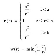
The IMSL_ROBUST_COV function computes robust M-estimates of the mean and covariance matrix from a matrix of observations. A pooled estimate of the covariance matrix is computed when multiple groups are present in the input data. M-estimate weights are obtained using the “minimax” weights of Huber (1981, pp. 231-235), with Percentage expected gross errors. Huber’s (1981) weighting equations are given by:
User specified observation weights and frequencies may be given for each row in x. Listwise deletion of missing values is assumed so that all observations used are “complete.”
Let f (x;µi, Σ) denote the density of an observation p-vector x in population (group) i with mean vector µi, for i = 1, ..., τ. Let the covariance matrix Σ be such that Σ = RTR. If:
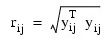
y = R-T (x - µi)
then:
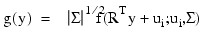
It is assumed that g(y) is a spherically symmetric density in p-dimensions. In IMSL_ROBUST_COV, Σ and µi are estimated as the solutions:

of the estimation equations:
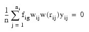
and:
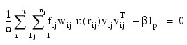
where i indexes the τ groups, ni, is the number of observations in group i, fij is the frequency for the j-th observation in group i, wij is the observation weight specified in column IDX_VARS(2) of x, Ip is a p by p identity matrix:
w(r) and u(r) are the weighting functions, and where β is a constant computed by the program to make the expected weighted Mahalanobis distance (yTy) equal the expected Mahalanobis distance from a multivariate normal distribution (see Marazzi 1985). The constant β is described more fully below.
The IMSL_ROBUST_COV function uses one of two algorithms for solving the estimation equations. The first algorithm is discussed in detail in Huber (1981) and is a variant of the conjugate gradient method. The second algorithm is due to Stahel (1981) and is discussed in detail by Marazzi (1985). In both algorithms, correction vectors Tki for the group i means and correction matrix Wk = Ip + Uk for the Cholesky factorization of S are found such that the updated mean vectors are given by:
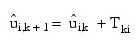
and the updated matrix R is given as:
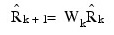
where k is the iteration number and:

When all elements of Uk and Tki are less than ε = TOLERANCE, convergence is assumed.
Three methods for obtaining estimates are allowed. In the first method, the sample weighted estimate of Σ is computed. In the second method, estimates based upon the median and the interquartile range are used. Finally, in the last method, you input initial estimates.
The IMSL_ROBUST_COV function computes estimates based on the “minimax” weights discussed above. The constant β is chosen such that E (u(r)r2) = ρβ where the expectation is with respect to a standard p-variate multivariate normal distribution. This yields estimates with the correct expectation for the multivariate normal distribution (for given mean vector). The expectation is computed via integration of estimated spline function. 200 knots are used on an equally spaced grid from 0.0 to the 99.999 percentile of:

distribution. An error estimate is computed based upon 100 of these knots. If the estimated relative error is greater than 0.0001, a warning message is issued. If β is not computed accurately (i.e., if warning message is issued), the computed estimates are still optimal, but the scale of the estimated covariance matrix may need to be multiplied by a constant in order for:

to have the correct multivariate normal covariance expectation.
Examples
Example 1
The following example computes a robust variance-covariance matrix. The last column of the data set is the group indicator.
n_groups = 2
x = TRANSPOSE([[2.2, 5.6, 1.0], [3.4, 2.3, 1.0], $
[1.2, 7.8, 1.0], [3.2, 2.1, 2.0], [4.1, 1.6, 2.0], $
[3.7, 2.2, 2.0]])
cov = IMSL_ROBUST_COV(x, n_groups)
PM, cov, Title ='Robust Covariance Matrix'
Robust Covariance Matrix
0.522022 -1.16027
-1.16027 2.86203
Example 2
The following example computes estimates of the pooled covariance matrix for the Fisher’s iris data. For comparison, the estimates are first computed via IMSL_POOLED_COV. The IMSL_ROBUST_COV function with Percentage = 2.0 is then used to compute the robust estimates. As can be seen from the output, the resulting estimates are quite similar.
Next, three observations are made into outliers, and again, estimates are computed using functions IMSL_POOLED_COV and IMSL_ROBUST_COV. When outliers are present, the estimates of IMSL_POOLED_COV are adversely affected, while the estimates produced by IMSL_ROBUST_COV are close to the estimates produced when no outliers are present.
n_groups = 3
idxv = [1, 2, 3, 4] idxc = [0, -1, -1] percentage = 2.0
x = IMSL_STATDATA(3)
p_cov = IMSL_POOLED_COV(x, n_groups, Idx_Vars = idxv, $
Idx_Cols = idxc)
PM, p_cov, Title = 'Pooled Cavariance with No Outliners'
r_cov = IMSL_ROBUST_COV(x, n_groups, Idx_Vars = idxv, $
Idx_Cols = idxc, Percentage = percentage)
PM, r_cov, Title = 'Robust Covariance with No Outliners'
IDL Prints:
Pooled Cavariance with No Outliners
0.265008 0.0927211 0.167514 0.0384014
0.0927211 0.115388 0.0552436 0.0327102
0.167514 0.0552436 0.185188 0.0426653
0.0384014 0.0327102 0.0426653 0.0418816
Robust Covariance with No Outliners
0.247410 0.0872090 0.153530 0.0359695
0.0872090 0.107336 0.0538220 0.0321557
0.153530 0.0538220 0.170550 0.0411720
0.0359695 0.0321557 0.0411720 0.0401394
Syntax
Result = IMSL_ROBUST_COV(X, N_Groups [, BETA=variable] [, COV_EST=array] [, /DOUBLE] [, GROUP_COUNTS=variable] [, /HUBER] [, IDX_COLS=array] [, IDX_VARS=array] [, /INIT_EST_MEAN] [, /INIT_EST_MEDIAN] [, ITMAX=value] [, MEAN_EST=array] [, MEANS=variable] [, MINIMAX_WEIGHTS=variable] [, NMISSING=variable] [, PERCENTAGE=value] [, /STAHEL] [, SUM_WEIGHTS=variable] [, TOLERANCE=value] [, U=variable])
Return Value
Two-dimensional array containing the matrix of covariances.
Arguments
N_Groups
Number of groups in the data.
X
Two-dimensional array of size nrows by (n_variables + 1) containing the data where nrows = N_ELEMENTS(x(*,0)) and n_variables = (N_ELEMENTS(x(0,*)) – 1). The first n_variables columns correspond to the variables, and the last column must contain the group numbers.
Keywords
BETA (optional)
Named variable into which the constant used to ensure that the estimated covariance matrix has unbiased expectation (for a given mean vector) for a multivariate normal density is stored.
COV_EST (optional)
Two-dimensional array of size n_variables by n_variables containing the estimate of the covariance matrix. Keywords MEAN_EST and COV_EST must be used together.
DOUBLE (optional)
If present and nonzero, double precision is used.
GROUP_COUNTS (optional)
Named variable into which the one-dimensional array of length N_Groups containing the number of observations in each group is stored.
HUBER (optional)
If present and nonzero, Huber’s conjugate-gradient algorithm is used. The keywords STAHEL and HUBER cannot be used together.
IDX_COLS (optional)
One-dimensional array containing the indices of the variables to be used in the analysis.
IDX_VARS (optional)
Three element array indicating the column numbers of x in which particular types of data are stored. Columns are numbered 0 ... N_ELEMENTS(IDX_COLS) – 1.
- IDX_VARS(0) contains the index for the column of x in which the group numbers are stored.
- IDX_VARS(1) and IDX_VARS(2) contain column numbers of x in which the frequencies and weights, respectively, are stored. Set IDX_VARS(1) = –1 if there will be no column for frequencies. Set IDX_VARS(2) = –1 if there will be no column for weights. Weights are rounded to the nearest integer. Negative weights are not allowed.
-
Defaults: IDX_COLS= 0, 1, ..., n_variables – 1,
IDX_VARS(0) = n_variables,
IDX_VARS(1) = −1, and
IDX_VARS(2) = −1
INIT_EST_MEAN (optional)
If present and nonzero, initial estimates are obtained as the usual estimate of a mean vector and of a covariance matrix. The keywords INIT_EST_MEAN, INIT_EST_MEDIAN, and MEAN_EST cannot be used together.
INIT_EST_MEDIAN (optional)
If present and nonzero, initial estimates based upon the median and interquartile range must be used. The keywords INIT_EST_MEAN, INIT_EST_MEDIAN, and MEAN_EST cannot be used together.
ITMAX (optional)
Maximum number of iterations. Default: 30
MEAN_EST (optional)
Two-dimensional array of size N_Groups by n_variables containing initial estimates for the mean. The keywords MEAN_EST and COV_EST must be used together. The keywords INIT_EST_MEAN, INIT_EST_MEDIAN, and MEAN_EST cannot be used together.
MEANS (optional)
Named variable into which the array of size N_Groups by n_variables is stored. The i- th row of MEANS contains the group i variable means.
MINIMAX_WEIGHTS (optional)
Named variable into which the one-dimensional array containing the values for the parameters of the weighting function is stored. See the description at the beginning of this topic for details.
NMISSING (optional)
Named variable into which the number of rows of data containing missing values (NaN) for any of the variables used is stored.
PERCENTAGE (optional)
Percentage of gross errors expected in the data. Keyword Percentage must be in the range 0.0 to 100.0 and contains the percentage of outliers expected in the data. If the percentage of gross errors expected in the data is not known, a reasonable strategy is to choose a value of Percentage that is such that larger values do not result in significant changes in the estimates. Default: Percentage = 5.0
STAHEL (optional)
If present and nonzero, the Stahel’s algorithm is used. The keywords STAHEL and HUBER cannot be used together.
SUM_WEIGHTS (optional)
Named variable into which the one-dimensional array of length N_Groups containing the sum of the weights times the frequencies in the groups is stored.
TOLERANCE (optional)
Convergence criterion. When the maximum absolute change in a location or covariance estimate is less than Tolerance, convergence is assumed. Default: Tolerance = 10−4
U (optional)
Named variable into which an array of size n_variables by n_variables containing the lower matrix U, the lower triangular for the robust sample cross-products matrix is stored. U is computed from the robust sample covariance matrix, S (see the description at the beginning of this topic), as S = UTU.
Version History