You can enhance surface graphics by overplotting contour data to show more detail. In this topic, we will show two examples of using the SURFACE function along with the CONTOUR to display gravity and elevation data.
For an additional example using SURFACE, see Plot 3D Terrain and Water Table.
Example 1
For this example, we display simulated data for gravity measurements from a hypothetical meteorite impact crater in New South Wales, Australia. The data is stored in the file 'CraterGravityMeasurements.csv' in your IDL Examples/Data directory.
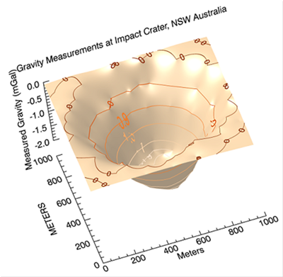
Since this is ungridded CSV data, read it in with your choice of ASCII readers. In this example we use READ_ASCII() with ASCII_TEMPLATE(). We will then grid the data before creating SURFACE and CONTOUR plots.
myTemplate = ASCII_TEMPLATE()
grav = READ_ASCII('CraterGravityMeasurements.csv', TEMPLATE=myTemplate)
grid = GRIDDATA(grav.x, grav.y, grav.z, DIMENSION=1000, METHOD="Kriging")
mySurf = SURFACE(grid, RGB_TABLE=16, TRANSPARENCY=25, COLOR='burlywood', $
XTITLE="Meters", YTITLE="METERS", TITLE="Gravity Measurements at Impact Crater, NSW Australia")
zAxis = AXIS('Z', LOCATION=[0, 1010], TITLE='Measured Gravity (mGal)', $
TICKINTERVAL=0.5, AXIS_RANGE=[-2.0,0.0])
mySurf['axis2'].TRANSPARENCY=100
contours = CONTOUR(grid, C_VALUE=grav.z, PLANAR=0, /OVERPLOT)
Example 2
This example works with digital elevation data from the Maroon Bells Wilderness in Colorado, USA.
The code shown below creates the graphic shown above. You can copy the entire block and paste it into the IDL command line to run it.
RESTORE, FILEPATH('marbells.dat', $
SUBDIRECTORY=['examples', 'data'])
mySurface = SURFACE(elev, TITLE='Maroon Bells Elevation Data')
myContour = CONTOUR(elev, N_LEVELS=15, $
/ZVALUE, PLANAR=0, /OVERPLOT)
Note: The ZVALUE keyword will not have any visual effect unless PLANAR is set to 0 and the plot is in a 3D dataspace, such as in conjunction with the SURFACE function.
Resources